Red-black trees (part 3)

published: Thu, 13-Mar-2008   |   updated: Fri, 5-Aug-2016

In this continuing series on red-black trees, we've now seen how to insert into a normal binary search tree. In fact the implementation and code were so simple, it's hard to even recognize that anyone would want to do anything else. Why invent more complicated binary trees, when the binary search tree seems to do so well?

The operative word there is "seems". In essence, in the previous episode, I had two simple tests with the binary search tree: the first was a carefully crafted program that created a complete binary search tree (remember a complete tree is one in which all the levels are filled, including the bottom level, and is automatically perfectly balanced), and the second was a mega stress test that added a lot of items in as random an order as I could make them.

Let's look at that last binary search tree. It contains about 2000 integers, added in a random order. What does that tree "look" like? I'm certainly not going to try and draw it. If it were perfectly balanced it would have 11 levels, with the last level not quite complete. If it were complete that last level would have 1024 items in it. I'm sure you'll agree that's going to be one large tree, when printed horizontally.

So let's approach it in a different manner. Let's calculate the shortest depth, the largest, and the average. This will give us an idea of the "bushiness" of the tree. If there's a wide spread between the shortest, the average, and the longest, there will be a wide variation in the length of the paths, and we can say the tree will be "twiggy", if the spread is small, all paths will be roughly the same length and we can say it's "bushy", or, if you like, balanced. We can easily calculate the average depth for a fully balanced tree and if the average for our tree is significantly larger, then that points to some twigginess too.

However there's a slight issue. Normally when we talk of the depth of a node we have this vision of taking a walk from the root to a leaf node, that is, a node with no children at the bottom of the tree. But there could well be nodes in the middle with only one child, and if one of those nodes were close to the root, it is an indication that the tree is not very well balanced. What we'll do instead is to calculate the length of the path from the root to each null child link in the tree. These null links are assumed to point to "external nodes". These nodes are not part of the tree per se, but just aid us in understanding how the tree works. (With red-black trees, the external nodes are very important, since they are always assumed to be black.)

This path length, if you think about it in terms of insertion, is the number of comparisons you have to make in order to insert a new item, since the new node is added to replace one of these external nodes. So the path lengths we'll be discussing here are the lengths of the paths for search misses.

Another fascinating fact is that if there are N internal nodes in the tree (internal nodes hold the items of information we are storing in the tree), then there are always N+1 external nodes. This is easy to prove: for N nodes there are 2*N links. Each internal node, except the root, has one of those links coming from its parent. So the number of links that go to an external node is 2*N - (N-1), or N+1. To put it another way, there are N+1 paths in the tree since each path goes from the root to an external node. The average path length for a "perfectly balanced" tree is log₂ of the number of paths if it is complete, or close to log₂ of the number of paths if it is not complete.

(Aside: instead of having null nodes as external nodes, we could create a single external node and have all the null links point to this node instead. Doing this can make some implementations of binary search trees easier to deal with, especially the red-black tree.)

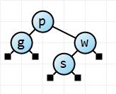
Here's an example. I changed my display routines so that the null nodes are shown as little black boxes.

Using it, we can see that the depth of the null node to the left of g is 2, as is the depth of the null node to the right. The depth of both null nodes for s is 3, and the depth of the external node at w is 2. There are 5 paths in total, the sum of the path lengths is 12, and so the average is 2.4. If we work out log₂ of 5 (paths) for the average for a perfectly balanced tree we get 2.32 (note that it cannot be complete, nor really perfectly balanced).

Let's just see a quick example of adding 15 items at random to a binary search tree.

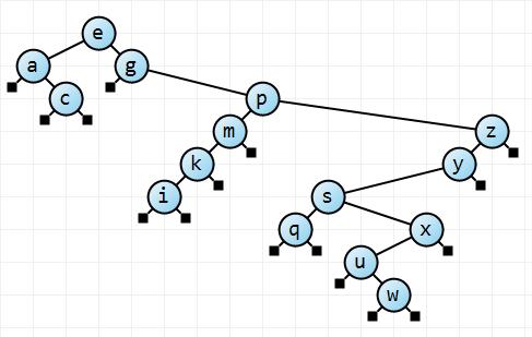
Here we have 2 paths of length 2, 2 of length 3, 2 of 4, 2 of 5, 2 of 6, 3 of 7, 1 of 8, and 2 of length 9. A total length of 87 units over 16 paths, which gives an average of 5.4. The perfectly balanced tree has an average path length of 4. From this little example, we see that the average path length has increased by about a third, and the minimum path length is 2 and the maximum is 9. We could rightfully conclude that our simple statistics correlate what we see: the tree is not very balanced, and you could argue it's downright twiggy.

In fact, as you play with this post's tree display program a little bit, you'll see that if you're dead unlucky with the very first item you insert you could get a very skewed tree. In particular, if the first item you insert is close to — or is! — the smallest or largest item then the tree will be very skewed either to the right or to the left subtree of the root. In this scenario, the root is killing the capabilities of the tree, since most paths will require that extra step, and comparison, from the root to the highly populated subtree.

Having played around with the tree display program, we can now run a few tests by inserting 2047 integer items in random order into a binary search tree and calculate the statistics. (For a complete binary search tree with 2047 internal items, the average search path is 11.) To be honest, I'm not interested in writing a statistical package for this series on red-black trees, so I merely exported the data over several runs to a CSV (comma separated values) file and imported it into Excel to play around with.

Actually I'll admit I was a little surprised at the results, never having done this exercise before. They were kind of interesting. Over 100 runs, with 2047 internal nodes inserted (and therefore 2048 possible paths to external nodes), the average shortest path was 4.3, the average longest path was 25.9, and the average of the average path lengths was 14.5. What this says to me is that adding random values to a binary search tree generally results in a reasonably well balanced tree; not brilliant exactly, but OK. The longest path lengths though are worrying, since they're usually well over twice as long as the "optimal" path length. But the average path lengths stay pretty reasonable, generally about 3 or 4 units longer than the optimum 11.

Notice though what this means: if you have inserted 2047 items in random order into a binary search tree hoping for a well-balanced tree, and then try and insert new items into that tree using the standard algorithm, on average you will be performing 3 or 4 more comparisons per search miss than you would do if the tree were perfectly balanced. That's about a third more, actually quite a lot. (For a derivation of this result, see Sedgewick's Algorithms in C (Third Edition), pp. 508-509.)

Next time, we'll look at how to improve these figures by using a red-black tree.

C# Source code. VB Source code. Note that this is a work in progress. These links merely point to the state of the code after part 3. There is a lot more to come.

[This is part 3 of a series of posts on red-black trees. Part 1. Part 2. Part 4. Part 5. Enjoy.]